MI-Sim A MATLAB Package for the Numerical Analysis of Ecological Motifs

• Home
• Installation
• Getting Started
• Documentation
• Glossary
• Thermodynamics module
• GUI Interface
• Examples
• Algorithms

Contents

• Screenshot
• Description
• Menus
• Models
• Plots
• Simulation
• Reporting
• Options
• Panels

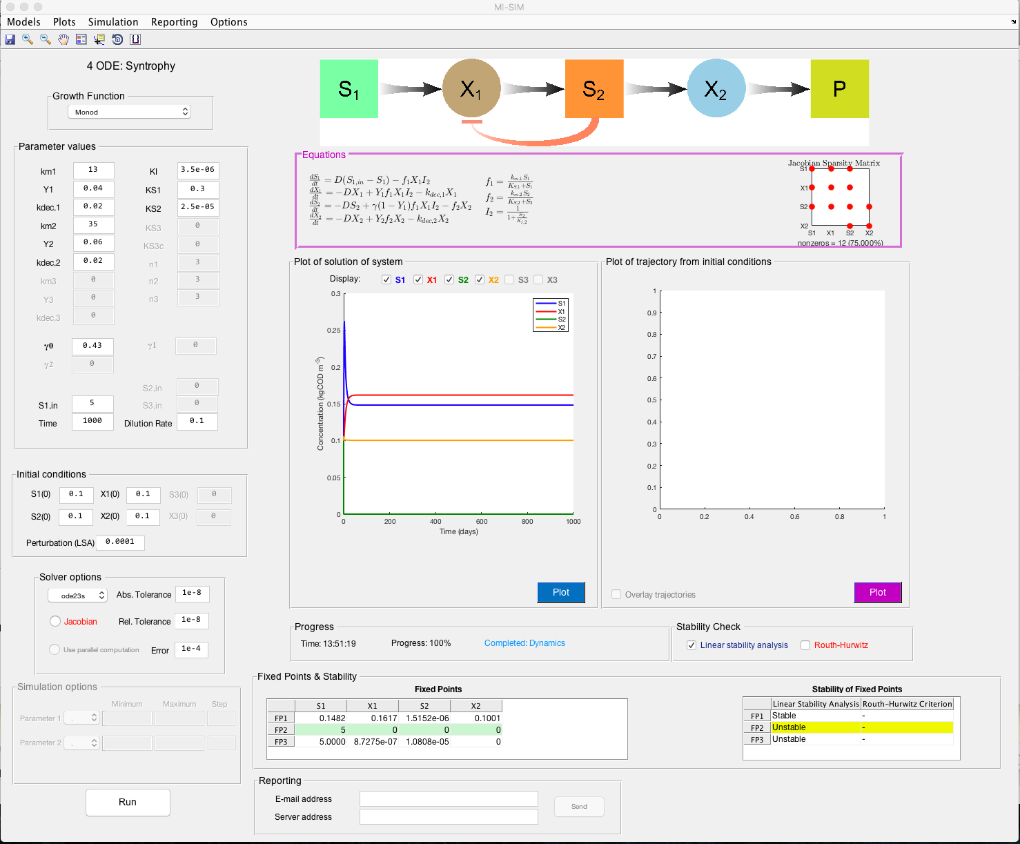
Screenshot

Description

Mathematical modelling of ecological interactions is affected by the model objective (e.g., observation, prediction, control), the knowledge available to inform the model and the structural complexity necessary to adequately describe the system or motif, and numerous analysis methods exist, accordingly. The software we present here focuses strictly on a mechanistic understanding of ecological interactions and, specifically, the analysis and simulation of microbial ecology networks for two or three species and associated substrates. However, the software is generic and the tools may be utilised for other ecological networks. The motif models are developed as systems of Ordinary Differential Equations (ODEs), which are used to describe the dynamics of and interactions between the individual biotic and abiotic components.

The MI-Sim software provides a user-friendly environment in which ecologists, biologists and mathematicians can rapidly characterise the dynamics of two or three species ecological motifs robustly, without the necessity to develop their own code or understand the mathematical details of dynamical systems analysis.

Menus

Models

In this version of MI-Sim, six common ecological motifs describing interactions between two distinct species, plus one extended motif that consists of three interacting species are modelled. The seven motifs are simple networks commonly observed at both micro- and macro-scales, and provide a theoretical basis by which biologists and ecologists can understand and visualise ecological interactions.

The motifs included in MI-Sim are expressed as a series of ODEs for the concentration of each organism, $X_n$, and each substrate, $S_n$ (where $n$ denotes an index labelling each species). These ODEs describe the microbial growth, catabolic conversion processes, and species interactions within the system. The equations are developed using a standard mass-balance approach coupled with stoichiometric information describing the chemical transformation between reactants and products in the system.

The models currently available in MI-Sim are described as follows:

Food Chain

ODE model:

$\frac{dS_1}{dt} = D(S_{1,in} - S_1) - f_1X_1$

$\frac{dX_1}{dt} = -DX_1 + Y_1f_1X_1 - k_{dec,1}X_1$

$\frac{dS_2}{dt} = -DS_2 + \gamma(1-Y_1)f_1X_1 - f_2X_2$

$\frac{dX_2}{dt} = -DX_2 + Y_2f_2X_2 - k_{dec,2}X_2$

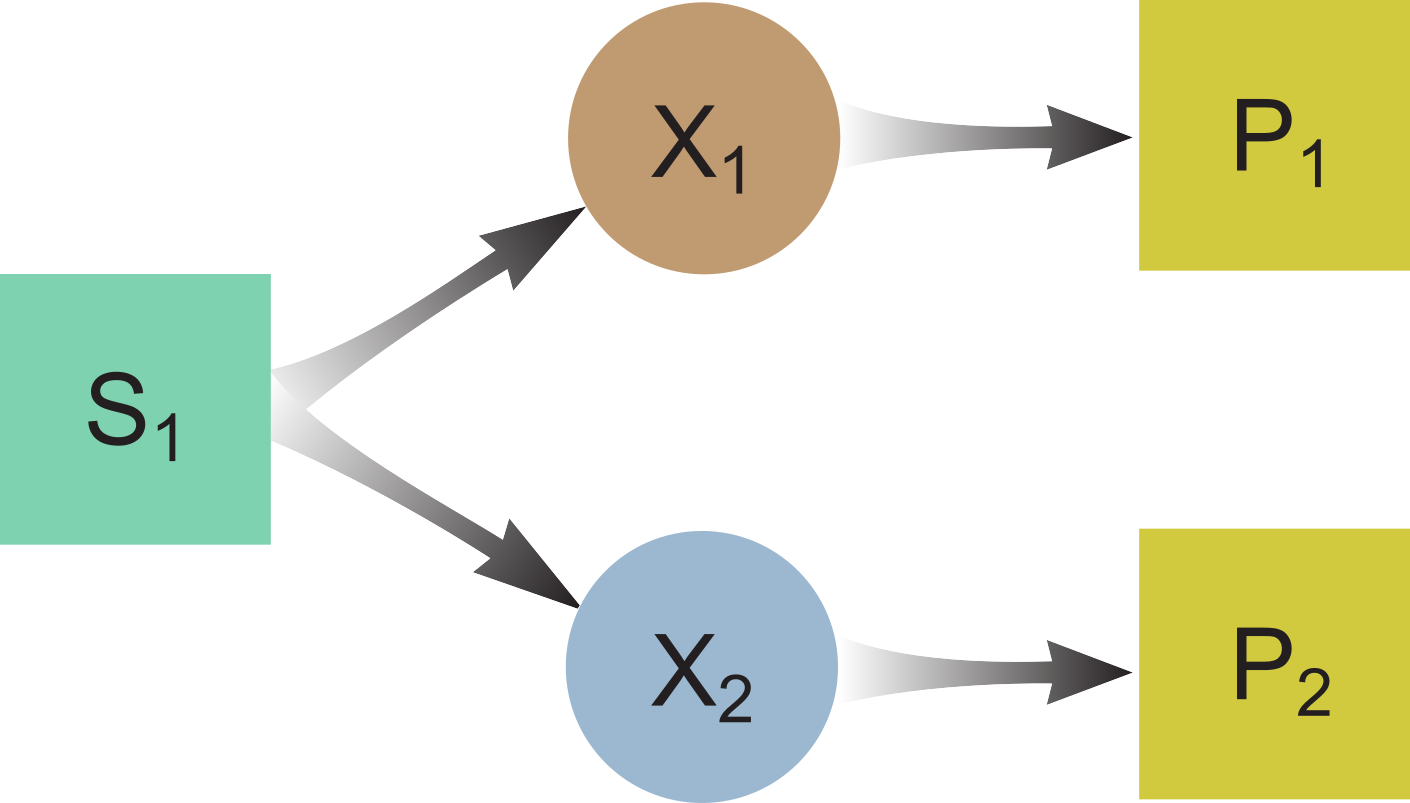
Substrate Competition

ODE model:

$\frac{dS_1}{dt} = D(S_{1,in} - S_1) - f_1X_1 - f_2X_2$

$\frac{dX_1}{dt} = -DX_1 + Y_1f_1X_1 - k_{dec,1}X_1$

$\frac{dX_2}{dt} = -DX_2 + Y_2f_2X_2 - k_{dec,2}X_2$

FC (Food Chain) with Product Inhibition

ODE model:

$\frac{dS_1}{dt} = D(S_{1,in} - S_1) - f_1X_1I_3$

$\frac{dX_1}{dt} = -DX_1 + Y_1f_1X_1I_3 - k_{dec,1}X_1$

$\frac{dS_2}{dt} = -DS_2 + \gamma(1-Y_1)f_1X_1I_3 - f_2X_2$

$\frac{dX_2}{dt} = -DX_2 + Y_2f_2X_2 - k_{dec,2}X_2$

$\frac{dS_3}{dt} = -DS_3 + f_2X_2$

$I_3 = \frac{1}{1+\frac{S_3}{K_{i,3,p}}}$

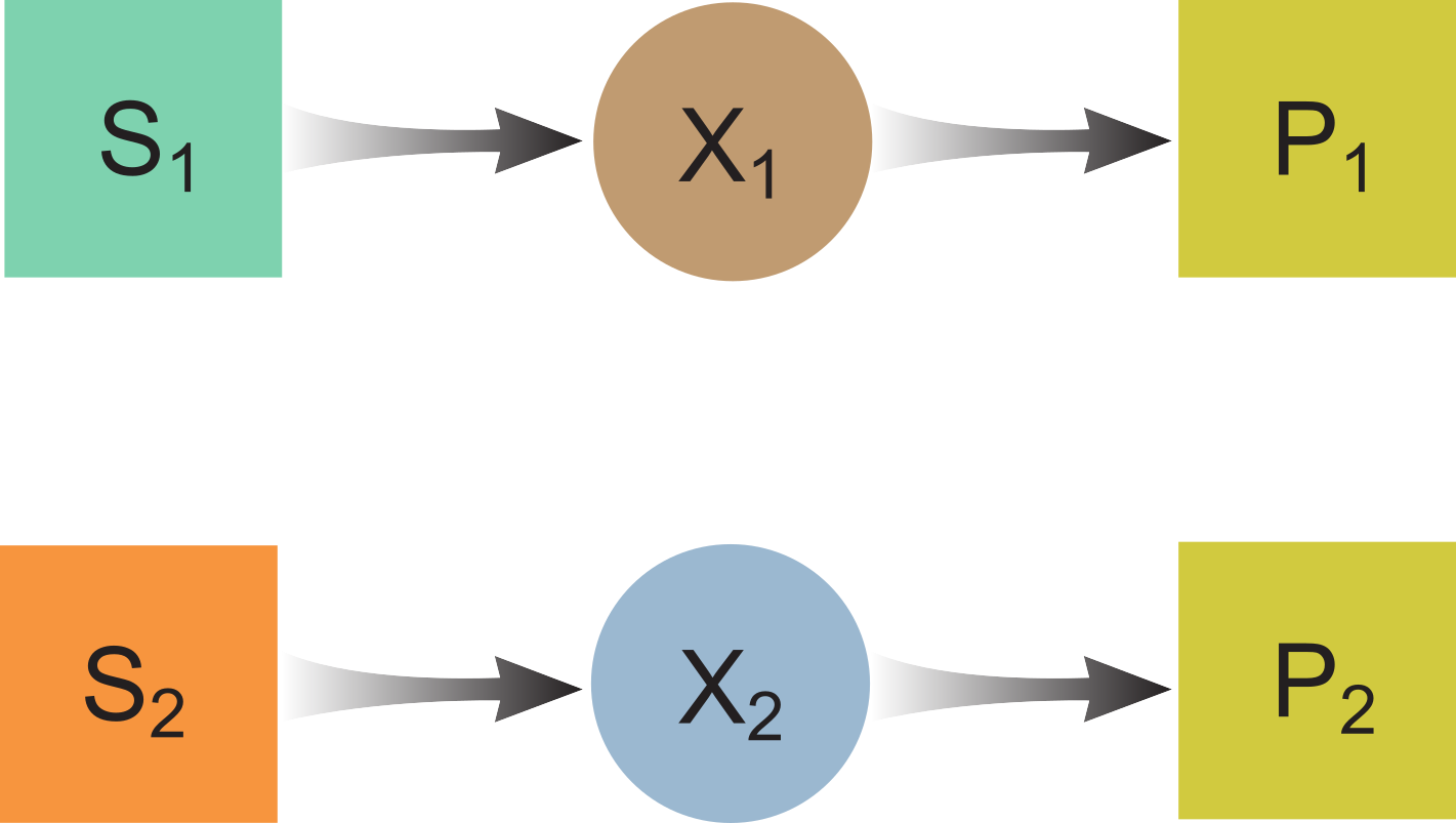
No Common Metabolites

ODE model:

$\frac{dS_1}{dt} = D(S_{1,in} - S_1) - f_1X_1$

$\frac{dX_1}{dt} = -DX_1 + Y_1f_1X_1 - k_{dec,1}X_1$

$\frac{dS_2}{dt} = D(S_{2,in} - S_2) - f_2X_2$

$\frac{dX_2}{dt} = -DX_2 + Y_2f_2X_2 - k_{dec,2}X_2$

Syntrophy

ODE model:

$\frac{dS_1}{dt} = D(S_{1,in} - S_1) - f_1X_1I_2$

$\frac{dX_1}{dt} = -DX_1 + Y_1f_1X_1I_2 - k_{dec,1}X_1$

$\frac{dS_2}{dt} = -DS_2 + \gamma(1-Y_1)f_1X_1I_2 - f_2X_2$

$\frac{dX_2}{dt} = -DX_2 + Y_2f_2X_2 - k_{dec,2}X_2$

$I_2 = \frac{1}{1+\frac{S_2}{K_{i,2,p}}}$

Waste Product Inhibtion

ODE model:

$\frac{dS_1}{dt} = D(S_{1,in} - S_1) - f_1X_1$

$\frac{dX_1}{dt} = -DX_1 + Y_1f_1X_1 - k_{dec,1}X_1$

$\frac{dS_2}{dt} = -DS_2 + \gamma(1-Y_1)f_1X_1$

$\frac{dX_2}{dt} = -DX_2 + Y_3f_3X_2I_2 - k_{dec,3}X_2$

$\frac{dS_3}{dt} = D(S_{3,in}-S_3) - f_3X_2I_2$

$I_2 = \frac{1}{1+\frac{S_2}{K_{i,2,p}}}$

Three species (Food-web)

ODE model:

$\frac{dS_1}{dt} = D(S_{1,in} - S_1) - f_1X_1$

$\frac{dX_1}{dt} = -DX_1 + Y_1f_1X_1 - k_{dec,1}X_1$

$\frac{dS_2}{dt} = D(S_{2,in} - S_2) + \gamma_0(1-Y_1)f_1X_1 - f_2X_2I_2$

$\frac{dX_2}{dt} = -DX_2 + Y_2f_2X_2I_2 - k_{dec,2}X_2$

$\frac{dS_3}{dt} = D(S_{3,in}-S_3) + \gamma_1(1-Y_2)f_2X_2I_2 - f_3X_3 - \gamma_2f_1X_1$

$\frac{dX_3}{dt} = -DX_3 + Y_3f_3X_3 - k_{dec,3}X_3$

$I_2 = \frac{1}{1+\frac{S_3}{K_{i,2,p}}}$

Growth functions

The growth functions defined, generically, as $f_p$ in the ODE models may take any rational form. At present, MI-Sim includes several common growth functions such as Monod, Contois, and Moser (see the QuickStart guide).

The following growth functions are currently included with MI-Sim:

Monod

$$f_{p} = \frac{k_{m,p}S_n}{K_{S,n,p}+S_n}$$

Contois

$$f_{p} = \frac{k_{m,p}S_n}{K_{X,p}X_n+S_n}$$

Moser

$$f_{p} = \frac{k_{m,p}S_n^{\lambda_n}}{K_{S,n,p}+S_n^{\lambda_n}}$$

Tessier

$$f_{p} = k_{m,p}(1-e^{-\frac{S_n}{K_{S,n,p}}})$$

Haldane

$$f_{p} = \frac{k_{m,p}S_n}{K_{S,n,p}+S_n+K_{i,2,p}S_n^2}$$ $$I_2 = 1$$

Andrews

$$f_{p} = \frac{k_{m,p}S_n}{K_{S,n,p}+S_n+\frac{S_n^2}{K_{i,2,p}}}$$ $$I_2 = 1$$

Thermodynamic

$$\Delta G = \Delta G^0 + RT\ln\left(\frac{\prod_{\nu=1}^{n_\nu}{S_\nu^{m_o}}}{\prod_{\pi=1}^{n_\pi}{S_\pi^{m_o}}}\right)$$ $$I_2 = 1-\exp\left(\frac{\Delta G}{RT}\right)$$

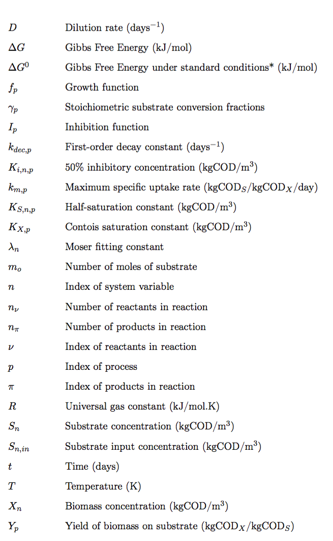
Description of symbols

*1 M concentration, 1 atm, 25$^\circ$C, pH 7

Plots

Two plot windows are available on the interface for visualisation of the analysis outputs. The plot menu provides options for how the figures are presented in the GUI.

Solutions

This option defines what is visualised in the left-hand plot window.

• Time-series - The dynamic profile of the variables from single-point analysis.
• Phase - A phase plot that visualises the dynamic trajectory of two or three variables. The check-boxes are used to select which variables will be plotted.
• Subplots - Plots of each individual variable time-series.
• Eigenvalues - A plot of the real vs. imaginary parts of the fixed-point eigenvalues. This option is available if the Routh-Hurwitz (sign of eigenvalues) stability analysis was selected.

An overlay radio button may be checked to allow for an overlay of results from multiple simulations. When plotting the eigenvalues from the Routh-Hurwitz analysis, an option to normalise the plot is presented so that large values are scaled for ease of visualisation.

Trajectories

• 2D - A two-dimensional representation of the fixed-point trajectories using two variables selected with the check-boxes.
• 3D - A three-dimensional representation of the fixed-point trajectories using three variables selected with the check-boxes.

These options also apply to the Phase Portrait analysis.

Toolbar

A toolbar provided below the menu options provides a number of plot manipulation tools. These include standard MATLAB functions such as save, zoom and legend. A bespoke button enables the current plot to be undocked from the GUI for further editing of the figure.

Simulation

Single-Point

This routine is used for analysing the dynamics and steady-state stability of the motif at a single point in the model parameter space. A description of the algorithm is provided here.

Multiple-Point

This is an extension of the single-point routine in which the stability analysis is performed for a range of user-specified values for any given parameter pair. The resulting steady-state regions and their stability are visualised as a two-dimensional bifurcation phase plane. This is a powerful method for understanding the relationship between model parameters and the existence and stability of the system steady-states. A description of the algorithm is provided here.

Basin of Attraction

For any pair of variables, the basin of attraction is determined by assessing the influence of their initial conditions on the steady-state reached. Ecological systems can exhibit multiple stable states within the same parameter space. In other words, depending on the initial conditions, a system may tend towards different equilibrium points representing distinct biological behaviour. A description of the algorithm is provided here.

Phase Portrait

The phase portrait algorithm is an alternative approach for visualising the location of state attractors. Unlike the basin of attraction analysis, this routine shows the trajectories of the solutions for the system of ODEs. A description of the algorithm is provided here.

Reporting

The reporting option allows the user to compile a PDF document of the output from the analyses performed during a single GUI session. A UI window displays a list of all available images (in PDF format) from which the user can select which to include in the PDF report. The file ‘date parameters.pdf’ contains a snapshot of the model parameters and equations, and should always be selected together with the image files. An Archive Reports will store previously generated reports in the ‘Reports/Archives/’ folder, and Delete Reports will remove all reports in the ‘Reports/’ folder and all images in the ‘temp_fig/’ folder. The user may e-mail this report using the E-mail address and Server address input boxes in the Reporting panel on the GUI.

Options

Three options are available to handle the interface status:

• Reset values - resets the parameter and simulation values to their default values
• Restart GUI - resets the entire GUI to the start-up state
• Close GUI - closes the GUI window

Panels

MI-Sim includes a number of panels that partition the interface functionally and in a logical manner. Other non-interactive text and graphical elements are included to inform the user about the motif under analysis.

All analyses are initiated using the Run button, whilst the Plot buttons will update plots after selection of options from the Plots menu.

Growth function panel

The dropdown growth function menu allows the user to select the growth model to be used in conjuction with the ecological motif. At present only Monod is included with the software, but future releases will cover a range of functions, as described here.

Parameter values panel

All parameter values may be entered manually by the user here. Only text boxes related to valid parameters for the selected model will be available and only non-negative numeric values will be accepted. The parameter symbols are generic, i.e. $k_{m,1}$, and their context can be determined by comparison with the model equations displayed in the Equations panel.

Initial conditions panel

For dynamical analysis of the model the starting concentrations of the model variables ($S_n$ and $X_n$) must be specified. The default values of $0.1$ kgCOD/m$^3$ are set at GUI initialisation. The Perturbation (LSA) text box is used to set the fixed-point perturbation value when Linear Stability Analysis is run.

Solver options panel

A number of in-built MATLAB ODE solver methods are provided here, with the default ode23s solver for stiff problems set at initialisation. The absolute and relative tolerance values may also be specified manually and act to control the error estimation of the algorithm for the given solver method (e.g., Rosenbrock formula of order two for ode23s). For non-trivial solutions, it may be necessary to adjust the tolerance values to improve accuracy, at the expense of simulation speed. A checkbox option Jacobian may reduce the stiff solver run-time by supplying a sparse Jacobian matrix to the solver. This avoids costly calls to the rate of change function. Further information on these solver options may be found here.

Simulation options panel

When a routine requiring simulation at multiple parameter or variable points is selected, this panel becomes active and the user may select which parameters or variables to investigate, their value ranges (min,max) and step-size. If Phase Portrait is selected, a 3D radio button is available to allow for selection between two- or three-dimensional visualisation of the phase trajectories.

Equations panel

The panels on the right side of the interface are specifically used for displaying information about the model systems and the results from the analyses. This panel displays the system of ODEs associated to the selected motif.

The Jacobian sparsity matrix is displayed when running fixed-point analysis routines on the right of the panel, whilst the central area is reserved for displaying a table of the existence-stability regions $\mathcal{J}$ after multiple-point analysis is complete.

Plot panels

Two figures are displayed to visualise the outputs from the software analyses. A description of the options for plot manipulation can be found in the Plots section.

Progress panel

For monitoring the progress of the different routines, this panel displays information on their percent completion. This may be for a single analysis, or for sub-routines within a multi-step analysis.

Stability check panel

Two options are available for performing stability analysis of the fixed-point solutions when running Single Point Analysis; Linear Stability Analysis and Routh-Hurwitz Criterion (for Multiple Point Analysis, Routh-Hurwitz is universally applied). Further details on these methods are found in the Algorithms section.

Fixed-points and stability panel

This panel displays the calculated fixed-point solutions and their stability for each variable. For Linear Stability Analysis the stability of the fixed-point may be either stable or unstable, whilst Routh-Hurwitz attempts to provide a more descripting classification of the fixed-points based on the type and sign of their eigenvalues.

Reporting panel

If the reporting option is selected, this panel allows the user to provide an e-mail address to which the PDF report can be sent. It is necessary to also provide a server address associated to the e-mail.

The e-mail should take the standard form:

yourname@yourserver.com

whilst the server should be written:

mail.yourserver.yournetwork